Uncategorized

Headstraps Considered Harmful for Cardboard-like VR Viewers

Disclaimer: I've been working on VR as a Product Manager at Google for a few years, and I was interested in the space for some time before that (e.g. see this). However, when push comes to shove: this is my personal blog and the views expressed on these pages are mine alone, and not those of my employer.

Since late 2014, accessible and simple smartphone-powered VR viewers like Google Cardboard brought the first taste of VR to larger audiences than ever before. In January 2016 Google has announced that over 5 million headsets have shipped.

Ever since the original Cardboard launch in 2014, there was one feature that puzzled the press and the users more than anything else: the lack of a headstrap.

Here's why including a headstrap with Cardboard-like devices wouldn't be a good idea.

VR presents a fundamentally difficult challenge of replacing the "natural" set of photons that would reach your eye from your surrounding environment with the set of "artificially" generated photons coming from the display. In order for you to feel comfortable in VR, this artificial set of photons has to approximate the behavior of the natural ones as closely as possible.

For example, when you turn your head, your brain expects the new set of photons to reach the eyes almost instantly. After all, this is how the real world always works.

Unfortunately, things in VR are slightly different.

To begin with, you don't actually need to get new visual input to know that your head position has changed. If you close your eyes and turn your head, your brain will get feedback from your neck muscles stretching and contracting, the tension on ligaments and tendons changing, the nerves in surrounding areas getting stimulated, angular acceleration being registered by vestibular system, and so on.

What this effectively means is that when you turn your head, your brain expects to receive the new set of photons because of proprioception. If there is a noticeable delay between your head movement and the new set of photons reaching your eyes, your brain realizes that something is wrong and copes with it using the oldest known trick in the book... Just like hundreds of thousands of years ago, if you ate the berries from the plant that you weren't supposed to and the toxins in the berries affected the levels of neurotransmitters, your brain would tell your body to get rid of the toxins in the fastest way possible: by making you throw up.

In VR's case, if the delay between the head movement and the new corresponding visual input exceeds 15-20ms (this delay is also known as motion-to-photon latency), you start experiencing the simulator sickness. Unfortunately, most of today's smartphones when used for VR, have the motion-to-photon latency of about 80-100ms.

This is because of two main reasons: the first reason is that today's smartphone operating systems have not been optimized for VR -- modern mobile OSes contain deep rendering stacks with double/triple buffering, no direct front buffer access, etc, which increase the time between the new frame being ready and the time when the new pixels are being sent to display. The second reason is that the underlying hardware components in the smartphones themselves also were not built for VR -- current smartphones ship with high-persistence displays (pixels take long time to switch on-and-off), low spatiotemporal resolution IMUs and so on.

So how does this all relate to the headstraps on Cardboard-like devices?

Well, turns out that the human peak angular neck velocity (~300 deg/s [1] [2]), is around 2-3 times faster than the peak angular torso velocity! (If you'd like to convince yourself, do a simple experiment: set a timer to 30 seconds and see how many times you can twist your neck side-to-side with your hands resting on your lap vs turning side-to-side with your hands held behind your head.)

By removing the headstrap and requiring the user to hold the viewer to their head with their hands, Cardboard-like devices effectively shift the user's yaw rotation plane from neck to torso, which in turn (pun intended) limits the maximum speed at which the user can change the position of their field of view, and masks the motion-to-photon latency.

Since reaching the peak angular velocities is definitely not a hypothetical scenario in VR (imagine if you were walking through a dimly-lit dungeon in VR and a zombie appeared in the periphery of your vision), reducing the speed of head movement to hide the motion-to-photon latency yields an better user experience overall: it's better to be forced to take small breaks at every 10 mins or so because your hands get a little bit tired than to constantly be experiencing the simulator sickness because of latency.

To end on a brighter note, the obstacles related to the smartphone motion-to-photon latency do not require any major technological breakthroughs: better hardware components can be put into the phones, and operating systems can be improved. As shown by Samsung Gear VR, when the motion-to-photon latency is reduced sufficiently, headstraps start making a ton of sense. In the meantime, the success of Cardboard-like devices also makes sense. They provide a simple way for the billions of existing smartphone users to understand what VR is about, to enjoy tens of thousands of "snackable" VR experiences already developed for the platform, and to share the fun with friends, family and colleagues.

References

[1] Bussone, Linear and Angular Head Accelerations in Daily Life. Master thesis at Virginia Polytechnic Institute and State University, USA, 2005.

[2] Öhberg et al. Chronic Whiplash Associated Disorders and Neck Movement Measurements: An Instantaneous Helical Axis Approach. IEEE Transactions on Information Technology in Biomedicine. 01/2004; 7(4):274-82.

 
135 Kudos
Don't
move!
Development, Work

"gcloud": Google Cloud Platform CLI for Power-Users

I tend to spend a lot of time in the command-line tools when working with the public cloud computing providers. It is fast, scriptable, and... strangely empowering.

Over the last year as a Product Manager on Google Cloud Platform, I have been thinking a lot about improving the developer experience. Obviously, one of the crucial parts of this experience is the command-line access to the cloud. To improve this experience, we have launched gcloud: a command-line tool for Google Cloud Platform, which enables developers to manage their Google Cloud-based resources in a consistent, uniform and efficient way.

I have captured the following video which showcases some of the power-use cases of gcloud that I am particularly excited about, and I think it may be worthwhile sharing. In particular, the video below features:

  • A single-line installation
  • Unified help
  • Command autocompletion
  • Remote resource autocompletion
  • Output formatting
  • Command chaining
  • Component management and updating
  • Access to the bleeding-edge commands, and so on.

The video is rather fast (apologies, but I wanted to keep it around 5 minutes), so you might want to pause it if you find something interesting.

Power use of gcloud: the CLI for Google Cloud Platform.

I hope you'll find it useful!

With that, I'm signing off from building next-generation cloud computing to building cheap, scrappy and accessible virtual reality.

Onwards and upwards, my friends!

 
111 Kudos
Don't
move!
Development, Life, Work

Google I/O 2014: Cloud and Android

It's obvious that cloud and mobile worlds are converging. The majority of interesting mobile applications nowadays are powered by cloud, and new startups are springing up every day to fight for their niche in this transition. Check out HN in your spare time; chances are you'll notice some new cloud-based data storage, a new way to test your apps in the cloud, or a new way to develop mobile apps using cloud-based IDEs. The importance of this convergence has even started changing the direction of old timers like Microsoft.

About a month ago, I had the opportunity to talk about some of the work I've been doing as a Product Manager on Google Cloud Platform to bring together the mobile and cloud worlds at Google I/O 2014. If you're curious to see how you could make your apps more engaging and more interactive using cloud without having to write hundreds of lines of code, check out the video of our session below.

Finally, as an added bonus, here are a few inside pictures from I/O 14! We live in the times of fundamental changes in computing and moonshot ideas, and it was a truly humbling experience to get a glimpse of that together with 6,000 in-person attendees at Moscone Center and over a million people who were watching the I/O keynote online.

 
148 Kudos
Don't
move!
Development, Education

Robot Photographer (Part IV, Final)

The story of Luke, an autonomous robot photographer, is officially completed and accepted to ICRA 2014!

The source code of the implemented robot photographer can be found at https://github.com/manfredzab/robot-photographer and the short description is below. If you need more technical information, take a look at my master's thesis, which contains all of the gory theoretical and implementation details, spread out over 140 pages.

All in all, developing Luke has been amazingly fun, but now it's time to move on to other exciting things. Silicon Valley awaits!

1. Background

Within the field of autonomous robotics and the variety of its application areas, robot photographers serve as excellent low-cost research platforms. They encompass a number of challenges common in robotics research, like task and path planning, locomotion and navigation (including obstacle avoidance), and human subject detection/tracking.

Robot photographers also include multidisciplinary challenges, like the automatic photograph composition (which requires computational understanding of the aesthetics of photography) or Human-Robot Interaction (HRI). As pointed out by Byers et al. [9], robotic photographer platforms are particularly well suited for HRI research, since the general public can easily grasp the overall concept ("it's a robot whose job is to take pictures"), and thus tend to interact with the robot naturally.

Finally, robot photographers show potential in commercial applications (e.g. event photography), since the service costs of an autonomous robot photographer are significantly smaller than those of a professional photographer.

Below a system is described that uses a single Microsoft Kinect sensor for obstacle avoidance and people detection, coupled with a consumer "point-and-shoot" camera for taking the final images, and which outperforms earlier robot photographer approaches.

2. Robot Photographer's Hardware

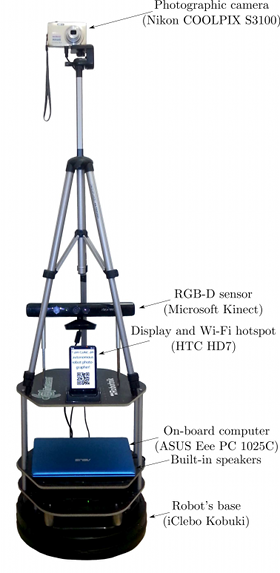
The developed autonomous robot photographer, Luke (shown below), is built using iClebo Kobuki's base, which has a 4kg payload, an operating time of around 3 hours, and maximum velocity of 65cm/s. Furthermore, Kobuki's base contains three bumpers (left, center and right) which can be used to provide alternatives to vision-based obstacle avoidance. This base is integrated into the Turtlebot 2 open robotics platform.

Luke: An Autonomous Robot Photographer

Luke: An Autonomous Robot Photographer

For its vision, Luke uses a Microsoft Kinect RGB-D sensor, which provides both a 10-bit depth value and VGA resolution color at 30 FPS. The sensor has a combined 57° horizontal and 43° vertical field-of-view.
The Kinect was attached to the Turtlebot's base at an inclination of 10° in order to be able to track upright standing humans at a distance of 1.5-2m. Since this limits low obstacle detection abilities, the linear velocity of the robot is limited to 10cm/s and the bumpers on Kobuki's base are used to provide graceful recovery in the case of collision with a low-lying obstacle.

To take the photographic pictures Luke uses a simple point-and-shoot Nikon COOLPIX S3100 camera, which has a maximum resolution of 14 megapixels, a built-in flash, and supports automatic exposure/ISO sensitivity/white balance settings. This camera is mounted on a lightweight, aluminium König KN-TRIPOD21 tripod (weighing 645 grams), which is attached to the top mounting plate of the robot. The overall size of the robot is approximately 34cm x 135cm x 35cm (W x H x D).

For Luke's state externalization, an HTC HD7 smartphone with a 4.3 inch LCD display was mounted onto the robot. The display has a resolution of 480 x 800 pixels, and is used to display Luke's state messages and to show the QR (Quick Response) codes containing the URLs of the pictures that Luke takes and uploads to Flickr. The smartphone also serves as a wireless hotspot, providing a wireless network connection between Luke's on-board computer and a monitoring/debugging station. Furthermore, it provides the internet connection to the on-board computer (for photo uploading to Flickr) by tethering the phone's 3G/EDGE connection over Wi-Fi.

The on-board ASUS Eee PC 1025C netbook has an Intel Atom N2800 1.6 GHz CPU and 1 GB RAM, providing a battery life of around 3 hours and weighs just under 1.25kg. It is running the Groovy Galapagos version of the Robot Operating System framework (ROS, [29]) on a Ubuntu 12.04 LTS operating system. All processing (including obstacle avoidance, human subject detection, photographic composition evaluation and so on) is done on this machine.

The robot contains two major power sources: a 2200mAh lithium-ion battery which is enclosed in the Kobuki's base, and a 5200mAh lithium-ion battery installed in the on-board netbook. Table below summarizes how these sources are used to power individual hardware components of the robot.

Hardware component Power source
On-board netbook Netbook's battery
Wheel motors Base's battery
Phone (display and Wi-Fi hotspot) Netbook's battery
Photographic camera Netbook's battery
Kinect RGB-D sensor Combined base and netbook's battery

During the empirical tests of the fully-powered robot, the average discharge times for the netbook's/Kobuki base's batteries were 3 hours and 6 minutes/3 hours and 20 minutes respectively.

3. Robot Photographer's Software

3.1. Architectural Design

Luke's software uses Brooks' [5] hierarchical levels-of-competence approach. Each of the layers in Luke's software hierarchy is based on the behaviors that Luke can perform:

  • The base layer allows Luke to aimlessly wander around the environment, while avoiding collisions.
  • The second layer suppresses the random wandering behavior at certain time intervals (adhering to what [5] called a subsumption architecture), and enables Luke to compose, take and upload photographs.
  • The final layer enables Luke to externalize his state i) visually, by showing text messages/QR codes on the attached display, and ii) vocally, by reading state messages out loud using text-to-speech software.
  • This architecture is illustrated in the following figure, and key implementation details are summarized below.
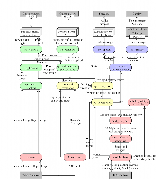
    A simplified Luke's architectural design diagram, showing ROS nodes (red, green, blue and yellow) together with I/O devices (gray rectangles), and the data that is being passed between them (text on the arrows). All nodes with prefixes rp_ (green, blue and yellow) are the results of the work described below, the red nodes are parts of Kobuki/ROS/GFreenect/Kinect AUX libraries. Yellow, green and blue nodes represent the first, second and third Luke's competence layers (corresponding to obstacle avoidance, human tracking/photograph taking and state externalization behaviors).

    A simplified Luke's architectural design diagram, showing ROS nodes (red, green, blue and yellow) together with I/O devices (gray rectangles), and the data that is being passed between them (text on the arrows). All nodes with prefixes rp_ (green, blue and yellow) are the results of the work described below, the red nodes are parts of Kobuki/ROS/GFreenect/Kinect AUX libraries. Yellow, green and blue nodes represent the first, second and third Luke's competence layers (corresponding to obstacle avoidance, human tracking/photograph taking and state externalization behaviors).

    3.2. Layer I: Random Walking with Collision Avoidance

    Luke's capability to randomly wander in the environment without bumping into any static or moving obstacles is implemented in three ROS nodes: rp_obstacle_avoidance, rp_locomotion and rp_navigation, as briefly described below.

    Obstacle detection and avoidance is based on [3], chosen due to its computational efficiency and suitability for the random navigation mode which Luke uses to wander around in the environment. It consists of three main steps:

    1. The input point cloud is obtained using the GFreenect library [27], and subsampled using a voxel grid filter.
    2. The Kinect's tilt angle is provided by the Kinect AUX library [13] which returns the readings from the Kinect's accelerometer at 20Hz, and with a flat-floor assumption used to tweak the subsampled point cloud.
    3. The region of interest (ROI) in front of the robot (defined by the user) is isolated from the transformed point cloud and a moving average of the ROI's size calculated. A positive average size generates a turn direction, otherwise the robot moves forward.

    To prevent the robot from getting stuck in an oscillating loop when facing a large obstacle, it is prohibited from changing the direction of the turn once it has started turning, as suggested in [3]. Also, an improvement from [28] is used whereby if the unfiltered point cloud is small then it is assumed that the robot is facing a nearby large obstacle, and a turn directive is issued.

    3.3. Layer II: Taking Well-Composed Photographs of Humans

    Luke's second major behavioral competence involves his ability to i) track humans in an unstructured environment, ii) take well-composed pictures of them, and iii) upload these pictures to an on-line picture gallery. This competence layer is implemented by five ROS nodes: rp_head_tracking, rp_framing, rp_camera, rp_uploading and rp_autonomous_photography.

    The head detection and tracking node (rp_head_tracking) is the most sophisticated node in Luke's ROS graph. For subject head detection it uses a knowledge-based method by Garstka and Peters' [18], which is extended to cope with multiple people presence in the image. To improve the head detection results, it employs one of the two skin detectors: a Bayesian skin detector by Jones and Rehg [22], and an adaptive skin detector based on a logistic regression classifier with a Gaussian kernel, and trained on an on-line skin model obtained from the face regions detected using the Viola and Jones [32] detector. Finally, to exploit the spatial locality of human heads over a sequence of frames, this node uses a depth-based extension of the continuously-adaptive mean-shift algorithm by Bradski [4].

    The multiple person extension still scans through a blurred and depth-shadow-filtered depth image one horizontal line at a time, from top to bottom. However, instead of keeping a single potential vertical head axis, a set of vertical head axes \{ H_1, ..., H_k \} is constructed. Each head axis is represented by H_i = \left( \overline{d}_i, (X, Y)_i \right), where \overline{d}_i is the average candidate head distance from the sensor, and (x, y) \in (X, Y)_i are the image points on the vertical axis.

    When a new arithmetic mean of left and right lateral gradients \overline{x}(y) is calculated in the original algorithm, the extended method searches for the head axis H_j such that the last added point (x', y') \in (X, Y)_j is within 5cm distance from the point (\overline{x}(y), y).

    If the pixel (\overline{x}(y), y) satisfies the above constraint then (X, Y)_j is updated by adding the point (\overline{x}(y), y), and the average head distance \overline{d}_j is recalculated.

    A vertical head axis H_i is classified as a detected candidate head if it is closer than 5m, is between 20-30cm tall, and is rotated by less than 35°. A few examples of multiple head detection using this method are shown in figure below.

    Multiple head detection examples

    Multiple head detection examples

    The detected candidate heads are verified using one out of two skin detection methods: a Bayesian classifier trained off-line on a very large scale skin/non-skin image dataset [22], and an on-line skin detector trained using skin histograms obtained from a small set of face detections using Viola and Jones [32] detector. In the first case a histogram-based Bayesian classifier similar to [22] is implemented and trained off-line on a large-scale Compaq skin dataset containing nearly a billion pixels, each hand-labelled as skin or non-skin.

    If this skin classification method is used, then a given candidate head detection is accepted/rejected based on the proportion of skin-color pixels in the corresponding RGB image region.

    In the second case, many faces are detected in the initialization stage using the frontal and profile face detectors using [32]. For each of the detected face rectangles, a binary mask is applied to segment the image into face oval/background regions, and the pixel hue histograms are assembled in each of the regions. Then these histograms are used as feature vectors in kernel logistic regression (KLR) classifier training. When this classifier is trained, the depth-based head detections can be verified by applying the same oval binary mask to the detected head rectangle, constructing a hue histogram from the face region, applying the KLR classifier, and thresholding.

    To further reduce the computational complexity requirements of head/skin detection methods described above, a depth-data based extension of the continuously adaptive mean-shift tracking algorithm (CAMShift, [4]) is employed to exploit the spatial locality of humans over a sequence of frames. While the original CAMShift algorithm uses the probability distribution obtained from the color hue distribution in the image, in this project it is adapted to use the depth information. In particular, the constraints that [18] use to reject local horizontal minima which could not possibly lie on the vertical head axis, are used to define the following degenerate head probability:

     \text{Pr}(\textit{head}\,|(x, y)) = \left\lbrace \begin{array}{cl} 1, & \text{if pixel }(x, y)\text{ is a local minimum} \\ & \text{in depth image and it satisfies the} \\ & \text{inner/outer head bound constraints}, \\ 0, & \text{otherwise}, \end{array} \right.

    which is then tracked using CAMShift.

    The second most important node in Luke's "picture taking" behavioral capability layer is the photograph composition and framing (rp_framing) node. This node works as follows. First of all, it subscribes to the locations of detected/tracked human subject heads in Kinect's image plane, published by the rp_head_tracking node. Then this node maps the head locations from Kinect's image plane to the photographic camera's image plane and calculates the ideal framing based on the framing rules described by Dixon et al. [12]. If the calculated ideal frame lies outside the current photographic camera's image plane, a turn direction is proposed; otherwise, the ideal frame location is published over /rp/framing/frame topic.

    In order to map the locations of detected heads from Kinect's to photographic camera's image plane, the rigid body translation vector is first established between the Kinect senor and the photographic camera. Then, the photographic camera is undistorted using a "plumb bob" model proposed by [6]. This model simulates (and hence can be used to correct) both radial distortion caused by the spherical shape of the lens, and the tangential distortion, arising from the inaccuracies of the assembly process. Finally, the approach of [34], [35] is used to estimate the camera intrinsics (viz. camera's focal length and principal point offsets). Then, any point in Kinect's world space can be projected into the photographic camera's image space.

    Using this approach, the 3D locations of the detected heads (provided by the rp_head_tracking node) are projected onto the photographic camera's image plane. Then, based on these locations the ideal framing for the photographs is calculated using the photograph composition heuristics proposed by [12]. These heuristics are based on the following four photographic composition rules [21]:

    • Rule of thirds, which suggests that the points of interest in the scene should be placed at the intersections (or along) the lines which break the image into horizontal and vertical thirds.
    • No middle rule, which states that a single subject should not be placed at a vertical middle line of the photograph.
    • No edge rule, which states that the edges of an ideal frame should not be crossing through the human subjects.
    • Occupancy ("empty space") rule, which suggests that approximately a third of the image should be occupied by the subject of the photograph.

    Given these rules, [12] define three different heuristics for single person and wide/narrow group picture composition. In order to choose which heuristic will be used they employ an iterative procedure. It starts by identifying a human subject closest to the center of the current image and calculating the ideal framing for this person using the single person composition heuristic. If this frame includes other candidate subjects, the group framing rules are applied iteratively on the expanded candidate set, until no new candidates are added.

    After an ideal frame F is calculated, the rp_framing node calculates the overlap coefficient between the part of the frame visible in the current image and the whole frame.

    If this exceeds a given threshold and the visible part of the frame exceeds the minimal width/height thresholds \theta_w \times \theta_h, the node considers that the satisfying composition has been achieved and publishes the position/size of the ideal frame over the /rp/framing/frame topic.

    Otherwise, the framing node determines the direction of where the robot should turn in order to improve the quality of the composition (based on the position of the ideal frame's center w.r.t. the image's center) and publishes these driving directions over the /rp/framing/driving_direction topic. In order to prevent the robot from getting stuck indefinitely while trying to achieve an ideal framing, a decaying temporal threshold for the minimum required overlap is also used. In the current robot photographer's implementation, the framing time limit is set to 60 seconds, the maximum deviation from the ideal overlap is set to 50% and the minimum visible frame size thresholds \theta_w \times \theta_h are set to 2160 x 1620 pixels.

    The rp_autonomous_photography node coordinates the actual photograph taking/uploading process, and divides the robot's control time between the obstacle avoidance (rp_obstacle_avoidance) and framing (rp_framing) nodes.

    The photograph taking node (rp_camera) acts as an interface between other ROS nodes and the physical Nikon COOLPIX S3100 camera that Luke uses to take pictures using the libgphoto2 API for the open-source gPhoto² library [2], which in turn connects to the camera using the Picture Transfer Protocol (PTP). This node provides access to the camera for the rest of the Luke's ROS graph by exposing a ROS service at /rp/camera/photo. Any other ROS node can send an empty request to this service, which rp_camera node transforms into the photo capture request for the libgphoto2 API. This request triggers a physical camera capture, storing the taken picture in the camera's built-in memory. After the picture is taken, rp_camera node moves the picture from the camera's memory to the on-board computer and returns the string file name of the downloaded picture via the service response.

    The photograph uploading node (rp_uploader) uses the Python Flickr API [31] to upload image files to an online Flickr photo gallery. It exposes the Flickr API to the rest of ROS graph by providing /rp/uploader/upload ROS service. The internet connection required for the picture uploading is provided by the on-board HTC HD7 phone (which also acts as a robot's state display) by tethering the phone's 3G/EDGE data connection over Wi-Fi to an on-board netbook which runs the overall Luke's ROS graph.

    3.4. Layer III: Externalization of the Current State via Vocal and Visual Messages

    Luke's third and final behavioral competence involves its ability to externalize its current state via synthesized voice messages (played over the on-board computer's speakers), and text messages/QR codes (shown on the display of the attached HTC HD7 phone). The state externalization node (rp_state_externalization) subscribes to the status outputs from all major nodes in Luke's ROS graph, in particular, the lomotion (rp_locomotion), head tracking (rp_head_tracking), framing (rp_framing) and photography process control (rp_autonomous_photography) nodes.

    In order to produce the robot's state messages (which are later vocalized/displayed by rp_speech and rp_display nodes) the state externalization node uses a table of pre-defined text messages, indexed by the states of four major nodes listed above. If the table contains more than one message for a given collection of states, then the message to be produced is chosen uniformly at random from the matching messages.

    In the current implementation, a HTC HD7 phone is used to show the received messages. This phone has a 4.3 inch, 480 x 800 pixel LCD display, and is running Windows Phone (WP) 7.8 operating system. To show the messages generated by rp_state_externalization node, a WP OS app connects to the rp_display node over TCP and renders received text messages in full-screen mode. If a hyperlink is present within the received text message then this app also generates and renders a QR (Quick Response) code. This makes it easier for the humans in the robot's vicinity to follow this link, since any modern phone can use the phone's camera to automatically read QR codes.

    To vocalize the text messages sent by rp_externalization node, the rp_speech node uses an open-source eSpeak [14] speech synthesis engine, which in turn is configured to use a formant synthesis based approach as described by Klatt [24].
    Since this method does not need a database of speech samples and uses computationally cheap digital signal filters, the resulting text-to-speech engine is both memory and CPU efficient, making it highly appropriate for the use in a mobile robot.

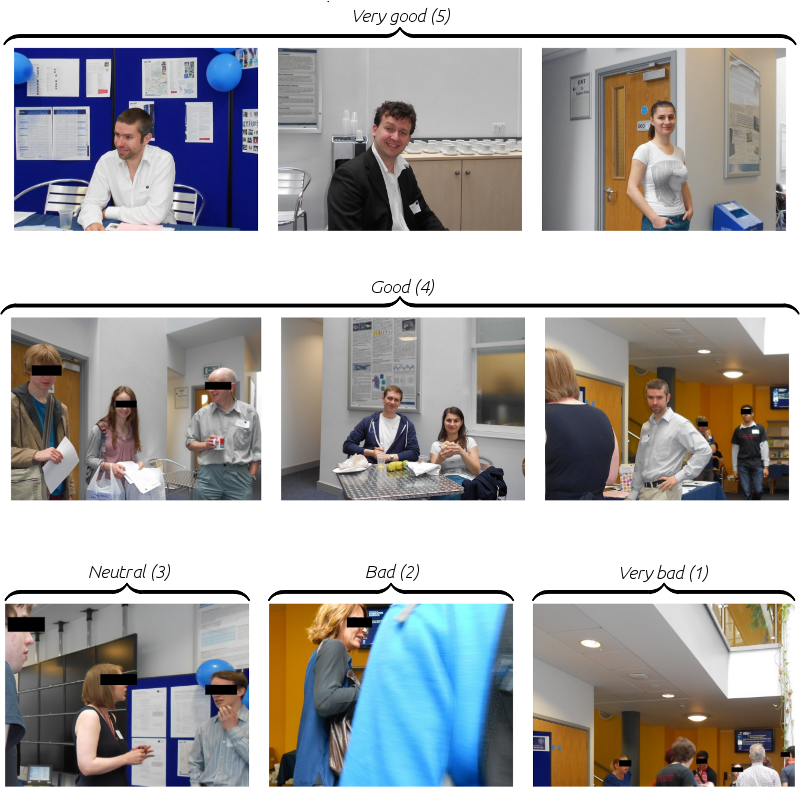
    A few examples of pictures taken by this robot together with the average ratings assigned by independent judges are shown in the figure below.
    Luke's photograph examples

    Luke's photograph examples

    4. References

    [2] Christophe Barbe, Hubert Figuiere, Hans Ulrich Niedermann, Marcus
    Meissner, and Scott Fritzinger. gPhoto2: Digital Camera Software,
    2002.

    [3] Sol Boucher. Obstacle Detection and Avoidance using TurtleBot
    Platform and XBox Kinect. Technical report, Rochester Institute of
    Technology, 2012.

    [4] Gary R Bradski. Computer Vision Face Tracking For Use in a
    Perceptual User Interface. Intel Technology Journal, (Q2):214–219,
    1998.

    [5] R Brooks. A Robust Layered Control System for a Mobile Robot.
    IEEE Journal of Robotics and Automation, 2(1):14–23, 1986.

    [6] Duane C Brown. Decentering Distortion of Lenses. Photometric
    Engineering, 32(3):444–462, 1966.

    [9] Zachary Byers, Michael Dixon, Kevin Goodier, Cindy M Grimm, and
    William D Smart. An Autonomous Robot Photographer. Intelligent
    Robots and Systems, 3:2636–2641, 2003.

    [12] Michael Dixon, C Grimm, and W Smart. Picture Composition for a
    Robot Photographer. Technical report, Washington University in St.
    Louis, 2003.

    [13] Ivan Dryanovski, William Morris, St´ephane Magnenat, Radu Bogdan
    Rusu, and Patrick Mihelich. Kinect AUX Driver for ROS, 2011.

    [14] Jonathan Duddington. eSpeak: Speech Synthesizer, 2006.

    [18] Jens Garstka and Gabriele Peters. View-dependent 3D Projection using
    Depth-Image-based Head Tracking. In Proceedings of the 8th IEEE
    International Workshop on Projector-Camera Systems, pages 52–58,
    2011.

    [21] Tom Grill and Mark Scanlon. Photographic Composition. American
    Photographic Book Publishing, Orlando, FL, 1990.

    [22] Michael Jones and James M Rehg. Statistical Color Models with
    Application to Skin Detection. International Journal of Computer
    Vision, 46(1):81–96, 2002.

    [24] D H Klatt. Software for a Cascade/Parallel Formant Synthesizer.
    Journal of the Acoustical Society of America, 67(3):971–995, 1980.

    [27] OpenKinect. GFreenect Library, 2012.

    [28] Brian Peasley and Stan Birchfield. Real-Time Obstacle Detection and
    Avoidance in the Presence of Specular Surfaces using an Active 3D
    Sensor. In 2013 IEEE Workshop on Robot Vision (WORV), pages
    197–202, January 2013.

    [29] Morgan Quigley, Brian Gerkey, Ken Conley, Josh Faust, Tully Foote,
    Jeremy Leibs, Eric Berger, Rob Wheeler, and Andrew Ng. ROS: an
    Open-Source Robot Operating System. In Proceedings of the 2009
    IEEE International Conference on Robotics and Automation, 2009.

    [31] Sybren A. Stuvel. Python Flickr API, 2007.

    [32] Paul Viola and Michael Jones. Rapid Object Detection Using a
    Boosted Cascade of Simple Features. In Proceedings of the 2001
    IEEE Computer Society Conference on Computer Vision and Pattern
    Recognition, pages 511–518, 2001.

    [34] Zhengyou Zhang. Flexible Camera Calibration by Viewing a Plane
    from Unknown Orientations. In Proceedings of the 7th IEEE International
    Conference on Computer Vision, pages 666–673, 1999.

    [35] Zhengyou Zhang. A Flexible New Technique for Camera Calibration.
    IEEE Transactions on Pattern Analysis and Machine Intelligence,
    22(11):1330–1334, 2000.

 
176 Kudos
Don't
move!
Development, Education

Robot Photographer (Part III)

The autonomous robot photographer is officially done, and it has already successfully completed its first real-world assignment!

The robot has been deployed during the open-days in Oxford's Computer Science Department. It ran for nearly three hours, taking 103 photos (approximately one photo every two minutes). A short video from this deployment is shown below.

Now, for some good news (at least for some of you, anyway). I will be producing a detailed write-up of robot's implementation as part of my Master's dissertation. As soon as that is completed (in a month or so), I will release both the dissertation and the source code for all software that is powering the robot! Given that the robot is built using low cost off-the-shelf hardware parts, I hope that it will enable some of you to create even more awesome autonomous robots!

Robot photographer development: real-world deployment

 
144 Kudos
Don't
move!
Development, Education

Robot Photographer (Part II)

A new milestone for the robot photographer! Here's a list of new things that the robot is capable of:

  • It has been taught to detect and track humans in Kinect's depth image!
  • Depth and photographic cameras have been aligned (camera intrinsics and extrinsics have been calibrated). This effectively means that given a point on one image plane (e.g. in the depth image), a robot is able to tell where the corresponding point would be on the other image plane (e.g. in a photograph).
  • Composition and framing modules have been implemented, i.e. now the robot knows how a "good" picture looks like.

All in all, this means that the "beta" version of the robot is now fully functional. Here's a new video of it in action!

Robot photographer development: human head tracking and picture framing

Next step: real world deployment!

 
150 Kudos
Don't
move!
Development, Education

Robot Photographer (Part I)

For a few weeks now I have been working on a new idea: an autonomous robot photographer.

My ultimate goal is to build a fully autonomous robot which could take well-composed pictures in various social events: conferences, open days, weddings and so on.

In the process I am also hoping to build a scalable system that could be extended to more complicated tasks and, potentially, used as a teaching tool at an undergraduate level.

I am planning to open-source both the software and the construction details, therefore I am using only widely accessible and inexpensive parts, and only open-source software.

My preliminary "ingredients" list for the robot includes:

  • a Microsoft Kinect sensor to detect humans and avoid obstacles in the environment,
  • a cheap point-and-shoot camera for taking the actual pictures, and
  • a Turtlebot spec compliant Kobuki robot base for the actual locomotion.

I will update the blog with more development details, but in the meantime, here's a video of the first development milestone: an autonomous navigation and obstacle avoidance.

Robot photographer development: obstacle avoidance

 
147 Kudos
Don't
move!
Development, Education

Expectation-Maximization Algorithm for Bernoulli Mixture Models (Tutorial)

Even though the title is quite a mouthful, this post is about two really cool ideas:

  1. A solution to the "chicken-and-egg" problem (known as the Expectation-Maximization method, described by A. Dempster, N. Laird and D. Rubin in 1977), and
  2. An application of this solution to automatic image clustering by similarity, using Bernoulli Mixture Models.

For the curious, an implementation of the automatic image clustering is shown in the video below. The source code (C#, Windows x86/x64) is also available for download!

Automatic clustering of handwritten digits from MNIST database using Expectation-Maximization algorithm

While automatic image clustering nicely illustrates the E-M algorithm, E-M has been successfully applied in a number of other areas: I have seen it being used for word alignment in automated machine translation, valuation of derivatives in financial models, and gene expression clustering/motif finding in bioinformatics.

As a side note, the notation used in this tutorial closely matches the one used in Christopher M. Bishop's "Pattern Recognition and Machine Learning". This should hopefully encourage you to check out his great book for a broader understanding of E-M, mixture models or machine learning in general.

Alright, let's dive in!

1. Expectation-Maximization Algorithm

Imagine the following situation. You observe some data set \mathbf{X} (e.g. a bunch of images). You hypothesize that these images are of K different objects... but you don't know which images represent which objects.

Let \mathbf{Z} be a set of latent (hidden) variables, which tell precisely that: which images represent which objects.

Clearly, if you knew \mathbf{Z}, you could group images into the clusters (where each cluster represents an object), and vice versa, if you knew the groupings you could deduce \mathbf{Z}. A classical "chicken-and-egg" problem, and a perfect target for an Expectation-Maximization algorithm.

Here's a general idea of how E-M algorithm tackles it. First of all, all images are assigned to clusters arbitrarily. Then we use this assignment to modify the parameters of the clusters (e.g. we change what object is represented by that cluster) to maximize the clusters' ability to explain the data; after which we re-assign all images to the expected most-likely clusters. Wash, rinse, repeat, until the assignment explains the data well-enough (i.e. images from the same clusters are similar enough).

(Notice the words in bold in the previous paragraph: this is where the expectation and maximization stages in the E-M algorithm come from.)

To formalize (and generalize) this a bit further, say that you have a set of model parameters \mathbf{\theta} (in the example above, some sort of cluster descriptions).

To solve the problem of cluster assignments we effectively need to find model parameters \mathbf{\theta'} that maximize the likelihood of the observed data \mathbf{X}, or, equivalently, the model parameters that maximize the log likelihod

 \mathbf{\theta'} = \underset{\mathbf{\theta}}{\text{arg max }} \ln \,\text{Pr} (\mathbf{X} | \mathbf{\theta}).

Using some simple algebra we can show that for any latent variable distribution q(\mathbf{Z}), the log likelihood of the data can be decomposed as
\begin{align}
\ln \,\text{Pr}(\mathbf{X} | \theta) = \mathcal{L}(q, \theta) + \text{KL}(q || p), \label{eq:logLikelihoodDecomp}
\end{align}
where \text{KL}(q || p) is the Kullback-Leibler divergence between q(\mathbf{Z}) and the posterior distribution \,\text{Pr}(\mathbf{Z} | \mathbf{X}, \theta), and
\begin{align}
\mathcal{L}(q, \theta) := \sum_{\mathbf{Z}} q(\mathbf{Z}) \left( \mathcal{L}(\theta) - \ln q(\mathbf{Z}) \right)
\end{align}
with \mathcal{L}(\theta) := \ln \,\text{Pr}(\mathbf{X}, \mathbf{Z}| \mathbf{\theta}) being the "complete-data" log likelihood (i.e. log likelihood of both observed and latent data).

To understand what the E-M algorithm does in the expectation (E) step, observe that \text{KL}(q || p) \geq 0 for any q(\mathbf{Z}) and hence \mathcal{L}(q, \theta) is a lower bound on \ln \,\text{Pr}(\mathbf{X} | \theta).

Then, in the E step, the gap between the \mathcal{L}(q, \theta) and \ln \,\text{Pr}(\mathbf{X} | \theta) is minimized by minimizing the Kullback-Leibler divergence \text{KL}(q || p) with respect to q(\mathbf{Z}) (while keeping the parameters \theta fixed).

Since \text{KL}(q || p) is minimized at \text{KL}(q || p) = 0 when q(\mathbf{Z}) = \,\text{Pr}(\mathbf{Z} | \mathbf{X}, \theta), at the E step q(\mathbf{Z}) is set to the conditional distribution \,\text{Pr}(\mathbf{Z} | \mathbf{X}, \theta).

To maximize the model parameters in the M step, the lower bound \mathcal{L}(q, \theta) is maximized with respect to the parameters \theta (while keeping q(\mathbf{Z}) = \,\text{Pr}(\mathbf{Z} | \mathbf{X}, \theta) fixed; notice that \theta in this equation corresponds to the old set of parameters, hence to avoid confusion let q(\mathbf{Z}) = \,\text{Pr}(\mathbf{Z} | \mathbf{X}, \theta^\text{old})).

The function \mathcal{L}(q, \theta) that is being maximized w.r.t. \theta at the M step can be re-written as
\begin{align*}
\theta^\text{new} &= \underset{\mathbf{\theta}}{\text{arg max }} \left. \mathcal{L}(q, \theta) \right|_{q(\mathbf{Z}) = \,\text{Pr}(\mathbf{Z} | \mathbf{X}, \theta^\text{old})} \\
&= \underset{\mathbf{\theta}}{\text{arg max }} \left. \sum_{\mathbf{Z}} q(\mathbf{Z}) \left( \mathcal{L}(\theta) - \ln q(\mathbf{Z}) \right) \right|_{q(\mathbf{Z}) = \,\text{Pr}(\mathbf{Z} | \mathbf{X}, \theta^\text{old})} \\
&= \underset{\mathbf{\theta}}{\text{arg max }} \sum_{\mathbf{Z}} \,\text{Pr}(\mathbf{Z} | \mathbf{X}, \theta^\text{old}) \left( \mathcal{L}(\theta) - \ln \,\text{Pr}(\mathbf{Z} | \mathbf{X}, \theta^\text{old}) \right) \\
&= \underset{\mathbf{\theta}}{\text{arg max }} \mathbb{E}_{\mathbf{Z} | \mathbf{X}, \theta^\text{old}} \left[ \mathcal{L}(\theta) \right] - \sum_{\mathbf{Z}} \,\text{Pr}(\mathbf{Z} | \mathbf{X}, \theta^\text{old}) \ln \,\text{Pr}(\mathbf{Z} | \mathbf{X}, \theta^\text{old}) \\
&= \underset{\mathbf{\theta}}{\text{arg max }} \mathbb{E}_{\mathbf{Z} | \mathbf{X}, \theta^\text{old}} \left[ \mathcal{L}(\theta) \right] - (C \in \mathbb{R}) \\
&= \underset{\mathbf{\theta}}{\text{arg max }} \mathbb{E}_{\mathbf{Z} | \mathbf{X}, \theta^\text{old}} \left[ \mathcal{L}(\theta) \right],
\end{align*}

i.e. in the M step the expectation of the joint log likelihood of the complete data is maximized with respect to the parameters \theta.

So, just to summarize,

  • Expectation step: q^{t + 1}(\mathbf{Z}) \leftarrow \,\text{Pr}(\mathbf{Z} | \mathbf{X}, \mathbf{\theta}^t)
  • Maximization step: \mathbf{\theta}^{t + 1} \leftarrow \underset{\mathbf{\theta}}{\text{arg max }} \mathbb{E}_{\mathbf{Z} | \mathbf{X}, \theta^\text{t}} \left[ \mathcal{L}(\theta) \right] (where superscript \mathbf{\theta}^t indicates the value of parameter \mathbf{\theta} at time t).

Phew. Let's go to the image clustering example, and see how all of this actually works. Continue reading

 
1135 Kudos
Don't
move!
Development, Education

3D Display Simulation using Head-Tracking with Kinect

During my final year in Cambridge I had the opportunity to work on the project that I wanted to implement for the last three years: a glasses-free 3D display.

1. Introduction

It all started when I saw Johnny Lee's "Head Tracking for Desktop VR Displays using the Wii Remote" project in early 2008 (see below). He cunningly used the infrared camera in the Nintendo Wii's remote and a head mounted sensor bar to track the location of the viewer's head and render view dependent images on the screen. He called it a "portal to the virtual environment".

I always thought that it would be really cool to have this behaviour without having to wear anything on your head (and it was - see the video below!).

My "portal to the virtual environment" which does not require head gear. And it has 3D Tetris!

I am a firm believer in three-dimensional displays, and I am certain that we do not see the widespread adoption of 3D displays simply because of a classic network effect (also know as "chicken-and-egg" problem). The creation and distribution of a three-dimensional content is inevitably much more expensive than a regular, old-school 2D content. If there is no demand (i.e. no one has a 3D display at home/work), then the content providers do not have much of an incentive to bother creating the 3D content. Vice versa, if there is no content then consumers do not see much incentive to invest in (inevitably more expensive) 3D displays.

A "portal to the virtual environment", or as I like to call it, a 2.5D display could effectively solve this. If we could enhance every 2D display to get what you see in Johnny's and my videos (and I mean every: LCD, CRT, you-name-it), then suddenly everyone can consume the 3D content even without having the "fully" 3D display. At that point it starts making sense to mass-create 3D content.

The terms "fully" and 2.5D, however, require a bit of explanation. Continue reading

 
410 Kudos
Don't
move!
Education

CST Part II

Nearly a year has passed since the last update. In order to at least partially rectify this situation, I am planning to publish a series of posts describing what have I been up to during that time. A natural place to start then is the final year of Computer Science undergraduate degree (also known as CST Part II) at Cambridge.

CST Part II undoubtedly offers a largest amount of flexibility out of all years of the Tripos. Three written exams (or as they are known in Cambridge, papers) have to be taken at the end of the year. Each paper contains fourteen questions, out of which five have to be selected and answered during a three hour exam.

This implies that it is enough to select a proper subset of subjects (out of twenty-four subjects offered in Part II) in order to do well in the final exams. This is where various strategies come into play.

Here is one that worked for me:

  1. Choose the courses that you are really interested in,
  2. Choose the courses that you are really good at.

The only remaining task then is to identify courses that satisfy the above criteria.

Let's start with #2: it is easy to be good at well-taught courses. That includes courses with well-written handouts, good exercise sheets and effective lecturers. Here is my list (but YMMW):

  1. All courses by Prof John Daugman (this typically includes "Information Theory and Coding" and "Computer Vision"). There are multiple good reasons for taking these courses: first of all, it is really worth seeing a polymath at work. I have not seen anyone closer to a Renaissance man than John Daugman. Secondly, the questions for ITC and CV follow the round-robin pattern over the years and never deviate from the material in the learning guides.
  2. "Business Studies" and "E-Commerce" courses by a serial entrepreneur-in-residence Jack Lang. I have been to a number of "business" courses, both within and outside the academic environment. I have not seen anyone eliminate the bullshit factor more effectively than Jack. This is both a tremendously effective skill to learn, and provides a very down-to-earth set of introductory lectures to anyone who aspires to be an entrepreneur. Exam-wise, Jack follows the same no-bullshit approach. The questions test your basic knowledge and provide an easy way to grab fifteen out of twenty marks (the median results for the year 2011-2012 were 15/20 for BS and 16/20 for E-C).
  3. "Computer Systems Modelling" by Dr Richard Gibbens. Besides the fact that Dr Gibbens is a very good lecturer, he is also very stable when it comes to setting the exam questions (viz. one out of two questions is always about the probability theory and the other is about queuing theory). Stability is predictability, and predictability is an expensive commodity in Cambridge exams.
  4. "Bioinformatics" (also known as "Algorithms III") by Dr Pietro Lio'. Despite sporting a couple of PhDs, Dr Lio' is a tremendously helpful lecturer. Seriously. He demonstrated it multiple times by arranging additional examples classes, Q/A sessions, handing out complementary lecture material and, of course, by setting the exam questions that yielded "very good results, well spread but with very few low marks" (his own words).
  5. Temporal Logic and Model Checking

    Temporal Logic and Model Checking scribbles...

    "Temporal Logic and Model Checking" by Prof Mike Gordon (not to be confused with the evil "Hoare Logic" course!). Behind the nasty notation hurdle (see the image on the right) lies another self-contained and straightforward course. This is also reflected in the exam results: the median marks for both TL&MC questions in 2011/2012 were 17/20!

Once again, the list above should be taken with a grain of salt, especially for the relatively young courses like Bioinformatics or TL&MC, where a large variance in the exam question difficulty has not been statistically disproved.

However, written papers account for only 75% of the final grade. The remaining 25% is allocated for the Part II dissertation. One of the biggest challenges in Part II is juggling between writing up the dissertation and learning for the exams, especially in the Easter term.

Here is my solution:

  1. Take all the courses in Michaelmas and Lent terms.
  2. Do not take any courses (apart from business ones) in the Easter term.
  3. Finish the implementation of the Part II project by the end of Christmas break. If you need to spend all your break on project work - do so; leave the revision for the Easter term (see below).
  4. Finish the write-up of the dissertation in the first two weeks of the Easter term. If you need to spend the whole Easter break on the dissertation work - do so.
  5. After the first two weeks of the Easter term you should be done with your dissertation and your courses (modulus a couple of business lectures per week). This means that between the first day of week three in the Easter term and the day minus-one of the first exam, you should be spending 95% of your time revising.

This approach has two main strength-points: first of all, the amount of task juggling is reduced to bare minimum. You work on your Part II project during the holidays, you study during the first two terms, and you spend all your time revising during the Easter term. Secondly, you avoid the "re-learning" (c.f. with Michaelmas courses in Parts 1A and 1B) since there is no new material between the revision and the exams to interfere. It tremendously reduces the amount of time required to prepare for 10-11 courses.

Finally, three tips for your revision:

  1. Go for the quality, not for the quantity. It is much better to have six strong questions in each paper than seven or eight average ones. Most people will go for the latter, making a huge mistake. Having four strong answers yields you a first class result while still leaving two questions for risk management.
  2. Find a suitable working space and establish a working regime. Separate "working" and "leisure" environments (e.g. work at the library instead of your college room). Seeing fifty people working hard around you both increases the motivation and decreases the temptation to procrastinate.
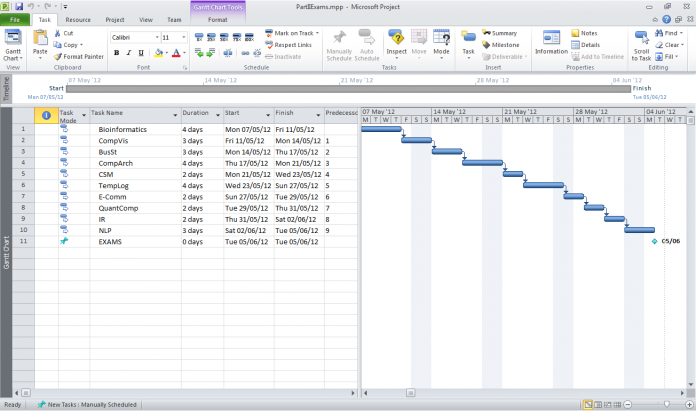
  3. Create a revision plan and follow it. Download Microsoft Project from DreamSpark and create a Gantt chart (you can see mine above). I am not joking. It is surprisingly easy to slip up by a day-or-two ("I will revise these two topics tomorrow and I will be done with the course.") Having an interactive schedule which can be easily updated, helps to see what trade-offs are actually being made ("I could revise these two topics tomorrow, but that will leave me only one day to revise the whole Information Retrieval subject").
gantt

Examination revision plan (Gantt chart in Microsoft Project)

International Undergraduate Awards 2012

So how does this all work in practice? For me this strategy yielded the average grade >80% (well above the first-class threshold) and a Jennings prize third year in a row. YMMW.

Perhaps more importantly though, it left me with enough time to do a Part II project that was highly-commended by the Computer Laboratory, and a >200 page dissertation that was highly-commended in the international 2012 Undergraduate Awards. More on the Part II project will follow in the later posts.

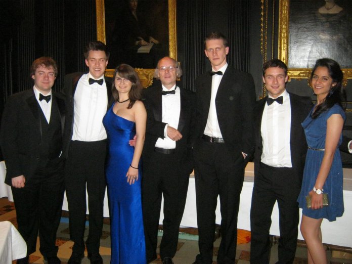
With Bjarne Stroustrup, creator of C++. Queens' College, Cambridge (2012 May)

It's not all doom and gloom. With Bjarne Stroustrup, creator of C++. Queens' College, Cambridge (2012)

 
217 Kudos
Don't
move!